
Every chart pattern score on StockDataAnalytics.com comes from a training pipeline that has run nearly 800 times since May 2026. It screens a few hundred candidate features per pattern, fits an additive model, tests it on a frozen holdout it never trains on, and marks a model ready for a live parallel run only if it beats the one already live on that holdout. One pass over all sixteen pattern detectors takes about three quarters of an hour on a single Mac (35 minutes when the samples were half the size). Ten of our twenty production detectors ran models that came out of it by mid-October.
Here is what surprised me when I stepped back and looked at what I had built. Most of the code is not modelling. The training tree is about 88,000 lines of Python, and the part that fits a model is a small slice of it. The rest is the ruler: the splits, gates and ledgers that decide whether a model is real. That is because the edge we are looking for is small. A typical fitted model's out-of-sample rank correlation with the two-week outcome is about 0.03; a good one reaches 0.08 or 0.09. At those sizes, telling a signal from a lucky draw of the data is the whole problem.
I spent 30 years building data platforms before this one, and it is the most self-measured system I have worked on. This article walks through what the pipeline does, in the order it does it, for the subscriber who wants to know what stands behind the score in the 6 AM email and for anyone building a trading model who wants to know where the traps are.
One caution belongs up front. The holdout numbers in this article are strong; the live numbers so far are not. On this year's production rows, measured within day and market at a one-week horizon, the pattern quality score has ordered market exposure rather than outcome, and only one detector in sixteen orders excess return the right way with an interval that excludes zero. The last section says what that means for the deploy rule.
Key facts
- 6,000+ NASDAQ and NYSE stocks scanned nightly for 16 bullish chart patterns
- Each detection scored 0 to 40 from three sub-scores: Structure, Volume and Breakout
- Up to 90,000 historical detections per pattern, January 2022 to March 2026, split 50/25/25 by date
- Nearly 800 training runs since May 2026; one run takes about three quarters of an hour
- Ten production detectors ran pipeline-trained models by mid-October
- The ten candidate models installed for parallel runs on October 15 won 61% to 82% of trades at scores of 36+ on their holdouts
What does the pipeline have to produce?
It has to produce a score where a 36 wins more often than a 24. If it does not, the ranking is noise and so is the email.
The scanner looks at about 6,000 stocks every night for sixteen bullish patterns: ascending triangles, bull flags, cup and handles, double bottoms, inverse head and shoulders, and eleven more. Each detection gets a quality score from 0 to 40 built from three sub-scores. Structure (0 to 15) covers the shape and context of the setup; Volume (0 to 12) covers what trading volume says about it; Breakout (0 to 13) covers the environment the pattern formed in. A two-week trade is simulated from the next morning's open, and subscribers get the top detections per market each day, ranked by score.
That product constraint shapes the design. The model cannot be an opaque forest of decision trees. A subscriber who sees a structure sub-score of 12 out of 15 is owed a 12 that is a sum of points from structure features, each pushing in a direction a person can follow. So the fitter is additive by construction, its output is a table of thresholds and points, and the production code it generates adds them up.
The target I set in spring was a top band that wins more than 75% of the time. In October I downgraded that from a gate to an aspiration, because absolute goals had started to block incremental progress. The gate now is a simpler question. Is this candidate better than what is live, on the worse of two out-of-sample windows, by enough to matter?
What happens in one training run?
One run takes each enabled detector (16 of 18 today) through the same chain, and a single detector's pass takes eight to ten minutes.
"Nightly" is a misnomer by now; a training batch is 20 to 40 iterations and runs through the day. On October 14 the history shows thirty runs.
Each detector's pass (a "leg") gets one strategy, which fixes the target (the measure of trade success the model is fitted to), the scoring mode and the market regimes it fits on; everything else is held constant, so two runs of the same strategy differ only by their random seeds. There are six targets to choose from, because the first one we used was wrong. A June post-mortem found that raw two-week return in a rising market is mostly beta (how much of the index's move a stock takes on): a model fitted to it could look predictive simply by liking volatile stocks. So the pipeline keeps six targets in play, among them return minus the index and a triple-barrier label (did the trade hit +1.5 ATR before −1.0 ATR within ten trading days).
The chain itself: pull a sample of detections and their outcomes; screen the candidate features; fit the model and translate it into a points ladder; ask whether the fit beats the best of many lucky tries; decide whether a read of the frozen holdout can resolve anything; read it; rate the result against the live model.
Here is a real leg from the run that produced one of the models installed on October 15: inverse head and shoulders, fitted to the triple-barrier label. Extract, 4 minutes. Feature screen, 2 minutes, 206 candidates left. Fit, 79 seconds, clearing the selection bar with an out-of-fold correlation of 0.0629. Holdout read allowed (seventeen earlier reads on that holdout, all logged). Live rule: the current model wins 54.5% at 36+; the candidate wins 71.6%. Deploy. Eight and a half minutes, start to finish. That is the unit of work, it is cheap, and taking many cheap shots is why most of the machinery below exists.
How is the data split, and why is the holdout frozen?
The split is one chronological cut: the oldest 50% of rows train the model, the next 25% validate it, the newest 25% is a holdout the model never sees until the final read, and the last 14 calendar days before each boundary are discarded so a two-week outcome cannot leak across.
Every training row is one detection (one stock, one day, one pattern) joined to the simulated trade that followed it. Almost every detector samples 90,000 rows from January 2022 to March 19, 2026. For the October 15 models, the cut worked out to training from early 2023 to August 2024, validation to mid-2025, and holdout from mid-2025 to March 2026.
The holdout is frozen: its rows are recorded by pattern, ticker and date, and every later extract rebuilds exactly those rows. The first version recorded database ids instead. A backtest deletes and reinserts the detections table with new ids, so a frozen holdout could silently shrink, and on September 22 it did: one detector's freeze matched 0 of 33,013 rows and nothing in the run said so. Now a freeze that resolves fewer than half its keys refuses to start the run.
Past the holdout sits a fourth slice, the forward period, which begins April 9, 2026. Training and the holdout read never load it; it is read once per promoted model, and by the parallel run.
How does the pipeline screen features?
Each candidate feature goes through fourteen checks, and the one that changed what the pipeline finds is a test of whether the feature predicts which stock to buy or merely when to buy.
Most of the battery is what you would expect: correlation with the outcome on training and validation, effect size between winners and losers, the same sign within bull and bear regimes and across chronological blocks, and a correlation with 20-day volatility no higher than 0.40, so the feature measures the pattern rather than the volatility class. One exclusion is deliberately loud. Any column whose name says it was measured over the outcome window raises an error and stops the run; four such columns were found in September. A feature that knows the future should stop the pipeline, not lose a tier.
The biggest change came in October, from a suspicion I had carried for months. Too many models leaned on market-wide features: index correlation, sector co-movement, the volatility regime. They predicted well in validation. I suspected the models were learning the calendar.
On October 5 we measured it on the seventeen models that had reached a holdout read. Each model's score spread was split into the part explained by which day a detection happened on and the part explained by ranking stocks against each other on the same day. The median validation win-rate spread between top and bottom score bands was 13.5 points; the within-date spread was 4.4; on the holdout both collapsed to about 2 points. Half of the validation spread was market timing, and the timing did not transfer.
Underneath that is an independence problem. The p-values had treated roughly 10,000 rows as independent observations. For a market-wide feature, every detection on one day moves together, so the real number of observations is closer to the number of trading days: around 400. Every significance test was overstated for exactly the features that transfer worst.
Three changes went in against it. A date-share gate rejects any feature with more than 30% of its variance between days. Significance is tested over days rather than rows: the correlation is computed within each trading day, and the mean of those per-day correlations is what gets tested. And the direction and consistency checks are recomputed on the same per-day statistics. The roster-wide admitted pool went from 1,407 features to 1,006, 28.5% fewer, each measured on the question that matters. With about 420 trading days in the window, the smallest within-day effect the screen can distinguish from zero is about 0.02, and only more days (not more rows per day) shrink that floor.
Multiple testing is controlled with the Benjamini-Hochberg procedure (which caps the share of false discoveries rather than the chance of any single one) at 10%. It replaced Bonferroni in June, because Bonferroni across a few hundred features had demanded p-values no real effect in this data reaches.
Why is the model additive, and how does it become a points ladder?
The model is a gradient-boosted tree ensemble constrained so hard that it stops being a forest: no tree may split on more than one feature, so the whole model is a sum of one-dimensional curves, and each curve can be read off as an exact table of thresholds and points.
For its first month the fitter tried the obvious workaround: fit an unconstrained "teacher" model and translate it into a ladder afterwards. The translation lost most of what the teacher learned. On May 29 the teacher went, and the fitter started fitting the ladder's shape directly.
Which features get in is decided twice. The screen's tiers are the first gate. The second is inside the fit, and it is where most features die: the fit is repeated nine times with different seeds, each time on the real features plus a shuffled "shadow" copy of every candidate, and a real feature is admitted only when its importance beats the 85th percentile of the shadow columns in at least five of the nine fits.
Cross-validation uses five contiguous date blocks, with training rows within 16 calendar days of a test block purged and the 10 days after it embargoed, and hyperparameters are re-tuned inside each fold.
Each component holds at most 12 structure, 10 volume and 10 breakout features, and the raw sums are scaled to the customer range by dividing by the 97th percentile of the training distribution. That percentile was 99.5 until October 4, and audits found that 419 of 421 fits never used the full score range: to reach 36, a detection had to sit near the 99.5th percentile on all three components at once, which almost nothing does. Lowering it changes no ranking; it only moves rows into the bands the deploy rule can judge. Finally the fitter generates the detector's scoring code, runs it in isolation against every row it was fitted and validated on, and requires a 100% match. The code that ships is the code that was tested.
How does the pipeline know a fit is better than luck?
Three tests must all pass: the fit's p-value survives correction against every earlier attempt on the same detector, its correlation beats the expected best of N random tries, and its top band beats the rest of the validation rows by more than a round-trip trade costs.
By October a busy detector had dozens of fits on the same data, and the best of fifty fits on noise will always look like something. The second test uses the Bailey and López de Prado approximation for the expected maximum of N draws, and N is not the raw count: earlier attempts are clustered by how similar their predictions are, so twenty near-identical fits count as fewer than twenty. The third test asks whether the top 5% to 10% of validation rows beat the rest by more than a 0.3% round-trip cost.
Two bugs in this bar show what "wrong" looks like here. Until July 3 the second test used the absolute value of the correlation, and a three white soldiers model with a correlation of −0.0634, ranking stocks backwards, passed with a z-score of +9.83. And until August 27 the third test asked only whether the top band's mean return was above zero; a bull flag model passed with a 410-row top band averaging 0.96% against a baseline of 1.12%. A band holding most of the population passes trivially, because its mean is the baseline. A gate audit in July counted 33 tests that could veto a model. Today exactly four can.
When is a holdout read worth spending?
A read is withheld when fewer than 50 holdout rows are projected to land in the top band, when the candidate's feature set overlaps 80% or more with the last model read on that holdout for the same target (unless its projected top band has grown by a quarter), or when the candidate's own validation numbers already fail the deploy rule.
Read a holdout fifty times and the best read is partly selected noise, so the pipeline treats each read as a resource. The projection of top-band rows used to be badly wrong: five of six audited reads in September were over-projected by 3.7 to 10.6 times, because a score cut chosen on validation lands much higher in the holdout distribution. The validation screen is the newest gate, and in its first stage it withheld 47 of 112 would-be reads: if a candidate cannot show 30 rows at 36+, a win rate above 50% and a spread above 5 points on its own validation window, it cannot pass on the holdout either.
How does a model get rated against the live one?
A candidate is rated on the worse of its validation and holdout windows, compared against the better of the production model and the model currently running in parallel, and it rates Deploy only if it wins more often at scores of 36 and above than the live model, shows a wider spread between its top band and its 20 to 24 band than the live model, and on its own numbers beats the market more than half the time at 36+ with a market-beat spread of at least 3 points. The production side is whatever model the last backtest scored the history with, so each push resets the bar to the model just installed.
Every holdout read is written to a registry before any holdout row is scored, with a fingerprint of the rows and a count of how many reads that holdout has seen. The read scores the holdout into a card: per integer score, the row count, win rate and market beat rate.
Until October 7 the final decision came from a tree of advisory labels and then a review by a language model. When I traced how models were actually being marked ready, a label reading "DEPLOY-CLASS: RANGE CARD FAIL" counted as ready because it started with "DEPLOY". So I wrote down how I judge a model by hand and made that the rule. It is the table below: eight conditions checked in order, each with the rating it produces, and the first condition the candidate matches decides. A candidate that trips none of the first seven is a Deploy.
| # | Condition | Rating |
|---|---|---|
| 1 | Fewer than 30 rows at 36+ in either window | Thin |
| 2 | Worse-window win rate at 36+ at or below 50% | Keep live |
| 3 | Holdout win rate at 36+ below the live model's by more than one standard error | Keep live |
| 4 | Holdout spread below the live model's by more than one standard error | Keep live |
| 5 | Worse-window spread under 5 points | Hold |
| 6 | Worse-window market beat at 36+ at or below 50%, or market-beat spread under 3 points | Hold |
| 7 | A tie with the live model, spread under 8 points, under 50 rows at 36+, or market beat under 53% | Deploy (caveat) |
| 8 | Otherwise | Deploy |
Deploy and Deploy (caveat) mark the model ready, and I install it in the parallel detector next to production; Hold, Keep live and Thin end the leg with the reason recorded. The spread is the win rate at 36 and above minus the win rate on the 20 to 24 band. The market-beat conditions in rows 6 and 7 came on October 12, after three of eighteen ready-rated models had won 55% to 63% of their trades at 36+ while beating the market only 41% to 47% of the time. A model that wins by riding the market is not doing its job.
What are the six ways a trading model fools itself?
Overfitting here is six separate problems with six different fixes, and the pipeline's history is largely the history of finding them one at a time.
1. Time leakage. Two detections ten days apart on the same stock share four days of price path. A shuffled split, which is what the pipeline started with, puts those rows on opposite sides of a fold and lets the model learn the future from its neighbours. Purged, embargoed folds close that. A subtler version hid until July 20: the fit's early-stopping set was the fold it was scored on.
2. Selection leakage. Fit fifty models and the best will look good whether or not any signal exists. Deflating for the number of attempts handles this within and across runs. Across holdout reads, I want to be plain about where things stand. After each read the pipeline computes a verdict deflated by the number of reads; it is recorded and gates nothing, and across the first four October versions of the pipeline it was false on 150 of 164 reads. A Deploy rating today is the best of many reads of one window. Keeping that advisory was a deliberate choice: produce candidates, and let the parallel run on live data be the arbiter, since that is a test no step of the search has seen.
3. Calendar leakage. The date problem above. One finding from it was counter-intuitive enough to record: subtracting a benchmark does not make a feature regime-neutral. The minus-market and minus-sector forms turned out to be the most date-driven family of all, because a stock's range variability minus its sector's still scales with the market's volatility regime.
The production evidence says the calendar defences are not finished. A separate analysis of this year's production rows, within day and market, found the model score's top quintile carrying a beta of about 1.0 against 0.4 to 0.7 in the bottom quintile in every period, while the beat rate across quintiles was flat or falling. A score that ranks beta will show a healthy raw win-rate spread on any holdout window in which the index rose, which is most windows drawn from the last two years, and lose it in the first window in which the index falls. The deploy rule measures raw win rate and raw market beat; it does not measure the exposure the top band carries relative to the bottom, and that number is computable on the holdout with no outcome data at all. Adding it, with a budget, and judging within-day ordering on beta-adjusted return are the next two changes to the rule.
4. Data-draw variance. Each night draws a different 90,000-row sample from a pool two or three times larger. We ran the same screen twice with only the data seed changed and 52% of the admitted features turned over; two models of the same detector trained on different draws shared 29% of their top-5% holdout picks. More rows helped (tripling the sample cut seed-to-seed churn on inverse head and shoulders from 96% to 38%), but the honest conclusion of that study is that "variance, not bias, dominates." The pipeline can fit the same detector five times and get five different models that all pass the same gates.
5. Holdout integrity. A frozen holdout protects nothing if it quietly stops being frozen, and ours broke five ways before it held, among them an integrity check that compared nothing with nothing and passed, the regenerated database ids described above, and a forward period that started on the day the training window ended, so the last two weeks of labels overlapped the "virgin" data.
6. Tooling leaks. On October 15, while testing candidate features for cup and handle with a research tool, we found that a column called close_at_rec was the close of the entry day, not the detection day. Any feature built against it contained one day of the future, worth a 20.8-point win-rate split between stocks on the same day. The leak was in the research tool, and it still overturned two research rounds. The heuristic that came out of it: a signal with the same sign on every detector in every period is more likely a leak than a law.
How small is the edge, and how does the pipeline see it?
The median model's out-of-sample correlation with the outcome is 0.031, and a good one reaches 0.08 or 0.09. Even at 0.05 to 0.10, the largest win-rate gap you can expect between a score of 30 and a score of 40 is 3 to 6 points, and the pipeline measures its own ability to detect effects that small by planting signals of known strength into real data.
For three months the pipeline produced nothing, because its gates were sized for effects that do not exist in this data. Flat-looking ladders in June were not a fitter failure. They were arithmetic. So the pipeline measures its own eyesight. A synthetic signal injector plants features with correlations of 0.03, 0.05, 0.08 and 0.12, plus pure noise columns, into a real dataset before the screen and reports what comes out. The first full probe in September, across ten detectors and ten seeds, gave the number that reset my expectations: the screen found planted correlations of 0.03 to 0.08 with no false positives in 249 null tests, and the selection bar was what failed. The pipeline could see the signal; it could not certify it. The rule that came out of it belongs at the top of any such tool: a gate change that moves the minimum detectable effect up is a sensitivity regression and needs an explicit decision, not a silent merge.
What moves the bar is breadth. An October 8 analysis of the best model per detector found that the spread in each model's weaker window rank-correlated +0.70 with its number of features and −0.68 with how concentrated its points were on a few features. Deploy-rated models averaged 14.6 features over 8.5 themes; Keep-live models averaged 3.7 features over 3 themes with 63% of their points on two. The strong models are not built from different features than the weak ones. They are built from more of them, spread more evenly.
What has the pipeline produced?
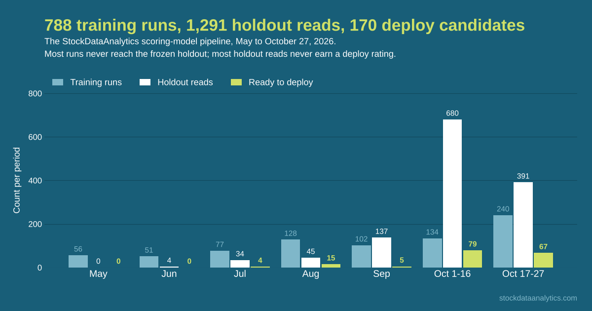
Since May the share of detector legs reaching a holdout read went from 5% to 37%, ready-for-deployment results spread from three detectors to thirteen, and ten models were installed on October 15 with holdout win rates at 36+ of 61.4% to 81.9%. The live production data tells a more sober story, below.
| Month | Runs | Detector legs | Holdout reads | Ready for deployment | Detectors with a ready model |
|---|---|---|---|---|---|
| May | 56 | 206 | 0 | 0 | 0 |
| June | 51 | 454 | 4 | 0 | 0 |
| July | 77 | 679 | 34 | 4* | 3 |
| August | 128 | 1,166 | 45 | 15 | 3 |
| September | 102 | 1,217 | 137 | 5 | 4 |
| October 1 to 16 | 134 | 1,826 | 680 | 79 | 13 |
| October 17 to 27 | 240 | 1,508 | 391 | 67 | 11 |
*The four July results were artifacts of a target pin and a bug in the bar. Holdout reads are counted from the touch registry from July 21 onward, and from run outcomes before the registry existed. The October 17 to 27 row includes the model-quality panel runs, which read the holdout under a tag; counts are as of the morning of October 27.
The table counts candidates. The next question is how good they were, and there are two answers: one for the ten models that were installed, and one for the whole October population they were picked from.
The ten models installed on October 15 were picked one per detector from recent holdout reads. On their holdout windows, their win rates at 36 and above ran from 61.4% to 81.9% (median 68.2%), spreads over the 20 to 24 band from 8.3 to 31.1 points (median 18.0), and market beat rates at 36+ from 54.0% to 71.3% (median 61.4%). Every one beats the market more than half the time at the top of its range, which the hand-built scores did not do.
Those ten are the top of a wide distribution. Of the October holdout reads with enough rows to be judged (440 as of October 16, with at least 30 rows at 36+ on both validation and holdout), the median holdout win rate at 36+ was 54.9% and the median spread 4.9 points, and those medians have sat there since September. The pipeline has become much better at producing candidates and at picking the best of them; it has not made the typical candidate better.
And the holdout cannot say how much of a top candidate's edge over the other candidates is real. Within a detector, the best read beats the median read by 12.0 points of win rate. With a run-to-run spread of 7.2 points, picking the best of the twenty to fifty reads a busy detector gets on one window would produce about 13.5 points from noise alone. Only the parallel run on live data can tell.
The live numbers so far are weaker than the holdout numbers, and I want that stated plainly rather than left to the limitations. The parallel runs are the real test, and the first read of them, on this year's production rows at a one-week horizon within day and market, is not what the holdout cards show. Pooled across detectors, the model score's beta rises monotonically from the bottom quintile to the top in every period while the beat rate is flat or falls; there is no period, at either horizon, in which the top quintile of the model score outperforms the bottom. Within each detector and day, the top-minus-bottom spread on excess return has a bootstrap interval excluding zero in the right direction for one detector of sixteen, and in the wrong direction for two or three. On this year's production rows the pattern quality score is an exposure ranker with no outcome ordering at the one-week horizon. The two readings can both be true: the holdout is a two-week horizon on windows in which the index mostly rose, and the live read is one week on a stretch that included a bad one. But a reader who finds both should know which one I weight. The live one. It is the reason the deploy rule is getting a beta-spread budget and a within-day, beta-adjusted ordering test, and the reason the calendar leakage section above calls those defences unfinished.
A plainer live view says the same thing with less precision. Taking the site’s own one-week evaluations of the daily top picks and cutting them at the dates new models were pushed to production (October 13 and 20): in the twelve trading days before the first push, picks won 43.0% and beat the market 45.1% of the time; in the five days after it, 58.5% and 55.4%. The before-window contains the bad week of October 6 to 13, when the market moved against high-beta names; without it, the before numbers are 48.6% and 46.2%, so the honest gap is about ten points of win rate and nine of market beat. The period after the push is the first encouraging read, and it is five days with no bad market day in it. Beta-adjusted favourable excursion (the best gain a pick reached during the week, net of the market) rose from 1.7% to 2.5% across the same cut. Whether that is better selection or more beta under another name is exactly what the within-day quintile study measures and this table cannot. The before-window holds about 550 picks and the after-window about 230, so the after-window win rate carries a standard error of roughly 5 points; I will refresh these once the second push has a week of its own.
What this means for you
If you are a subscriber: the score is a ranking instrument, and its value is in the spread between the top of the range and the bottom. A 38 is not a promise; it is a detection in the band where our out-of-sample win rate is highest. No model reaches production without passing a holdout it never trained on and a parallel run on live data, and the parallel run can still say no.
If you are building something like this: build the self-measurement first and the gates second. The pipeline was never short of signal. For three months it failed to certify signal of the size that exists, and when it finally certified models, many had learned the calendar. Both problems were invisible until the pipeline measured itself with planted signals, replays of past runs, and audits of its own projections against its own realised counts.
Limitations
The holdout has been read many times, and a Deploy rating is the best of many looks at one window. Variance between data draws is larger than I would like: five fits of the same detector can produce five different models that all pass. The deploy rule does not yet measure market exposure, and the live data says that is the gap that matters most. The figures here are as of pipeline version 2026.11.b, with funnel counts as of October 27; the parallel runs are still in progress as I write.
What comes next
Next in the queue: make the feature screen more stable across data draws, add a same-day version of every feature (each value minus that day's mean), and add a second sealed holdout read only as a confirmation for short-listed candidates. Not on the list, deliberately: loosening the volatility or date gates.
Frequently asked questions
How is a StockDataAnalytics pattern score calculated?
Each detection gets a 0 to 40 score that is the sum of three sub-scores: Structure (0 to 15), Volume (0 to 12) and Breakout (0 to 13). Each sub-score is a sum of points from a table of feature thresholds, fitted by an additive model on historical detections and their two-week outcomes.
How do you prevent overfitting in the scoring models?
Chronological 50/25/25 splits with 14-day purges, purged and embargoed cross-validation, a frozen holdout read only after a model clears a selection bar deflated for the number of prior attempts, a date-share gate that rejects features that predict timing rather than stock selection, and a parallel run on live data before any model replaces a production one.
What win rate do the trained models reach?
On their holdout windows, the ten models installed on October 15, 2026 won 61.4% to 81.9% of trades at scores of 36 and above (median 68.2%) and beat the market 54.0% to 71.3% of the time. Across all 440 October candidates the median holdout win rate at 36+ was 54.9%, so the installed models are the best of a wide distribution, and on live production data this year the score has ranked market exposure more reliably than outcomes.
How much historical data is each model trained on?
About 90,000 detections per pattern from January 2022 to March 2026, drawn from a daily scan of more than 6,000 NASDAQ and NYSE stocks, with each detection joined to a simulated two-week trade from the next day's open.